Wolters-Separability

2015-08-25

An R user who has done logistic regression more than a few times is likely to have seen this:

This warning may be accompanied by unexpectedly large/variable/unstable coefficient estimates, and an uneasy feeling that something is wrong with the model. The help for R’s glm function points the reader to Venables and Ripley (2002)¹, which, while being a very good book, isn’t particularly enlightening on this topic.

It isn’t hard to find discussions of this particular warning message online and in the academic literature, and the usual culprit is separability: there exists a plane in the covariate space that separates the “success” responses from the “failure” responses. When such a separation exists, the MLE of the regression coefficients does not exist (i.e., it contains infinities). If the separation condition is almost satisfied (sometimes called quasi-separability), it can still cause the coefficient estimates to have inflated variance, and can produce numerical difficulties in getting the estimates.

The statistical literature I’ve seen on this topic is (naturally) focused on how to get good parameter estimates, and as a result focuses on how to detect the separability problem, and how to remedy the situation to still get decent parameter estimates.

While these are important questions, my main motivation for writing this note is to approach this problem in the context of predictive modelling with large data sets: that is, using logistic regression to build a binary classifier. In this situation:

We’re fairly likely to get the above warning about fitted probabilities 0 or 1; especially if our classifier is working well.
We’re not particularly interested in the estimates of the regression coefficients, since it’s a pure prediction problem.

So the question we’re trying to answer is: If I get the above warning and/or inflated regression coefficients when building a logistic regression classifier, should I care? How do I know if I have a problem?

Setting the stage

We are doing logistic regression with a large collection of training data, say from $10^4$ to $10^6$ observations. The response vector is $\mathbf{Y}$ (the observed classes, taking values 0 or 1). We have $k$ vectors of observed predictors (a.k.a. features), $\mathbf{X}_1 \ldots \mathbf{X}_k$, where $k$ might also be large, perhaps in the hundreds or thousands (we might, for instance, have $m$ observed quantities and a large number of derived terms such as $X^{1/2}$ terms, $X^2$ terms, and various interaction terms).

This is what I call “biggish” data: the data set is large enough that we can’t ignore computational aspects, but it still can be held in the RAM of a single computer. We have many more features than we will ultimately need, so when we fit the model it’ll typically be as part of some sort of variable selection procedure (though I won’t talk about that part here).

Recall that the logistic regression model has

\[\mathrm{logit}(\pi_i)\equiv\log\left(\frac{\pi_i}{1-\pi_i}\right) = \mathbf{x}_i^T\boldsymbol{\beta} \equiv \eta_i,\]

where $\pi_i=\mathrm{P}(Y_i=1)$, $\mathbf{x}_i$ represents the length-$k+1$ feature vector for observation $i$, $\boldsymbol{\beta}$ is the vector of regression coefficients, and $\eta_i$ is called the linear predictor.

The goal here is to develop a classifier. To do this, we get the fitted regression coefficients $\hat{\boldsymbol{\beta}}$, compute the estimated probabilities $\hat{\pi}_i$, and assign case $i$ to class 1 whenever $\hat{\pi}_i > 0.5$ (we need not use 0.5 for this last step, but it’s reasonable to do so).

When we do this, we may observe one or more of the following:

We receive the glm.fit: fitted probabilities numerically 0 or 1 occurred warning when fitting the model.
The largest coefficient estimates are large, and variance estimates are also large.
The coefficient estimates are not stable, changing a lot when we fit with replicate data sets, or even when we change optimization convergence tolerances.

What causes the warning?

Fundamentally, the warning is caused by the finite precision of the computer’s arithmetic. After getting coefficient estimates, the fitted probability is

\[\hat{\pi}_i = \mathrm{alogit}(\hat{\eta}_i) = \frac{\exp(\hat{\eta}_i)}{1 + \exp(\hat{\eta}_i)}.\]

It is particularly easy to get the warning from large positive values of $\hat{\eta}_i$. When $\hat{\eta}_i$ is above about 40, the ratio on the right hand side will be within machine precision of 1. Negative values of $\hat{\eta}_i$ have to be much larger in absolute value to give a machine underflow and return exactly 0.

So usually, the warning can be taken to mean “there was at least one linear predictor over 40 or so.” This could have one of two causes:

We do have separation (or quasi-separation) of the responses by the predictors in the model. This has led to inflated coefficient estimates, which has caused some linear predictors to be large.
We don’t have a separation problem. Coefficients are well estimated, and we simply have some linear predictors $\hat{\eta}_i$ that are large enough in absolute value to give probabilities the machine can’t distinguish from 0 or 1.

The warning is perhaps more suggestive of the first cause in traditional statistical analyses, where the number of observations and predictors are smaller and there might be a lower signal-to-noise ratio in the data. In the biggish data classification problem, on the other hand, we hope and expect that our predictors have high discriminatory power, and that many observations will have large linear predictor values—that means those points are far from the decision boundary. So in that case it is more likely that the warning is due to the second cause, or a mixture of both causes.

Deciding what is really going on in a particular case, then, means diagnosing whether or not we have inflated regression coefficients.

What causes the effects on the coefficients?

Again, there are two possible causes to consider. The effects on the coefficients can arise:

When we have (quasi)separation, or
When the $\mathbf{X}$ matrix of covariates exhibits multicollinearity.

My primary reference on this issue has been Lesaffre and Marx (1993)². They refer to the quasi-separability problem as “ML-collinearity” and the usual multicollinearity problem as “collinearity”. ML-collinearity arises when the matrix $\hat{\mathbf{W}} = \mathbf{X}^T\hat{\mathbf{V}}\mathbf{X}$, which appears in the iteratively reweighted least squares (IRLS) iterates used to find $\hat{\boldsymbol{\beta}}$, is ill-conditioned; the ordinary collinearity arises when $\mathbf{X}^T\mathbf{X}$ is ill-conditioned. For logistic regression, the matrix $\hat{\mathbf{V}}$ is a diagonal matrix with $i$th element equal to $\hat{\pi_i}(1-\hat{\pi_i})$. So while collinearity depends on the predictors only, ML-collinearity depends on both the predictors and the response.

The paper defines $k_w$ and $k_x$ be the condition numbers of $\hat{\mathbf{W}}$ and $\mathbf{X}^T\mathbf{X}$, respectively, and $r_{wx}$ to be the ratio $k_w/k_x$ (note: they standardize the columns of $\mathbf{X}$ to unit length before computing the condition numbers). Lesaffre and Marx suggest the following rules of thumb based on these quantitites:

If $k_x > 30$, (ordinary) collinearity exists in $\mathbf{X}$.
If $r_{wx} > 5$ and $k_w > 30$, ML-collinearity (quasi-separability) exists.
If both of the above are true, both types of collinearity are occurring.

I have written an R function colincheck, provided at the end of the page, to compute these quantities for a given case.

The method of Lesaffre and Marx is handy, becuase 1) it allows us to determine when quasi-separability might be a problem, and 2) it lets us distinguish separability from run-of-the-mill collinearity among the predictors.

So how do I know if it’s a problem for my predictive model?

Now we can return to the original question: does any of this matter for building a logistic regression classifier? Unfortunately it’s not totally clear cut.

Some progress has been made in understanding the fitted probabilities numerically 0 or 1 warning. We can look at our linear predictors. The warning should be accompanied by at least some linear predictor values bigger than 40 or so.

At the same time, we can run colincheck to view the $k_w$, $k_x$, and $r_{wx}$ diagnostics of Lesaffre and Marx. This can tell us if we actually have collinearity and/or separability problems that will influence our regression coefficients.

There is still one missing link: if we do have collinearity of either kind, will this negatively affect our model predictions? Do we need to worry about the accuracy of our fitted probabilities? Unfortunately I am not aware of any theoretical answer to this question (such an answer may exist, I just haven’t seen it). I am inclined to conclude that in many cases, it is justifiable to ignore collinearity and quasi-separability issues when building a logistic classifier. My reasons for saying this:

Even if regression coefficient estimates are unstable and have high variance, the act of fitting the model will optimize discrimination between the two classes (a consequence of maximizing the likelihood). This assumes of course that the problem isn’t so bad that we have numerically singular matrices!
We are only interested in whether $\hat{\pi_i} > 0.5$ or $\hat{\pi_i} < 0.5$, so even some inaccuracy in fitted probabilities will not drastically impact the predictions.
I have observed the above two effects empirically when building models repeatedly using large samples drawn from an even larger population.

An R example

The code below can be used to generate an artificial data set with the characteristics we’ve been discussing. It generates a data set with $n$ observations and $m$ predictors. The predictors are generated in such a way³ that the correlation between any pair of $\mathbf{X}$ columns is $a^2/(1+a^2)$, where $a$ is a user-supplied constant. To generate a response vector, we assume that only the first $q$ predictors (after the intercept) are “active.” We set the first $q$ coefficients to take value $b$, while the remaining $m-q$ coefficients are zero.

Note, you’ll need to have the colincheck function from the bottom of the page loaded first if you want to try this code.

# Control parameters
n <- 1e4   #-Number of observations
m <- 100    #-Number of predictors
a <- 2     #-Controls correlation.  Correlation = a^2/(1+a^2).
b <- 1.5   #-Magnitude of active coefficients.
q <- 5     #-Number of active coefficients.

# Make model matrix
X <- matrix(0, nrow=n, ncol=m)  #-Initialize matrix.
w <- rnorm(n)                   #-Used only for creating correlation.
for(i in 1:m){
  X[,i] <- a*w + rnorm(n)       #-Make correlated X columns.
}
M <- cbind(rep(1,n), X)         #-Add the intercept.

# Make Y vector of responses
beta <- c(1, rep(b, q), rep(0, m - q))
eta <- M%*%beta
prob <- exp(eta)/(1+exp(eta))
Y <- rbinom(n, 1, prob=prob)

# Fit logistic regression (can be slow if n, m too large; recommend switching 
# to other packages, e.g. speedglm, for larger cases).
dat <- data.frame(class=Y, X)
fit <- glm(class ~ ., family=binomial(link="logit"), data=dat)

# Collinearity diagnostics
colincheck(fit)

# Estimated coefficients of active variables
fit$coefficients[2:6]

Running the code with the inputs shown gives the following output:

> fit <- glm(class ~ ., family=binomial(link="logit"), data=dat)
Warning message:
glm.fit: fitted probabilities numerically 0 or 1 occurred 
> 
> # Collinearity diagnostics
> colincheck(fit)
       kx        kw       rwx 
22.028758 11.072358  0.502632 
> 
> fit$coefficients[2:6]
      X1       X2       X3       X4       X5 
1.494141 1.496475 1.509190 1.691806 1.545439

Sure enough, we get the warning. Our colincheck diagnostics, however, suggest that we have neither collinearity or quasi-separability (all of $k_x$, $k_w$, and $r_{wx}$ are small). We can look at a histogram of the linear predictors using hist(fit$linear.predictors):

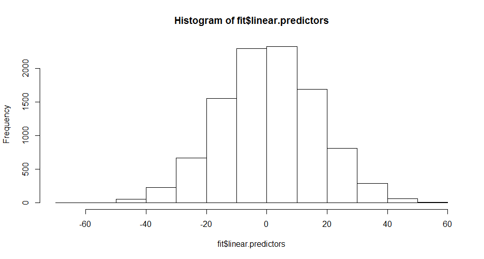
There are plenty of $\hat{\eta}_i$ values over 40, which explains why we saw the warning. So in this case we have little reason to suspect collinearity or separability problems: we simply have large linear predictors.

It is instructive to run the above code for different combinations of the inputs. You will find, for example, that increasing the number of predictors $m$, or increasing the correlation through $a$ will cause an increase in $k_x$ and result in inflated coefficient estimates. The larger coefficient estimates will in turn leading to a greater number of large-magnitude linear predictors.

Further remarks

A few final comments:

I haven’t commented on why or how the coefficient estimates become inflated when collinearity or ML-collinearity are present. This question is important for a deep understanding of this topic, but at the time of writing I am lacking both the time and ready knowledge required to answer it. It is more complicated than the linear regression case (where we have only one type of collinearity to consider, and we can use variance inflation factors to diagnose it) because logistic regression is a nonlinear model. For a correctly-specified logistic regression, the inflation should be due to an increase in variance, rather than bias. But for an overspecified or misspecified model, I believe bias can enter the picture.
Demidenko (2013)⁴ gives quite a detailed explanation of the separability problem for binary GLMs. He provides both necessary and necessary and sufficient critera for existence of the MLE, with algorithms for checking the conditions on a given data set. So it is possible to check definitively if the data are separable. There are a couple of caveats, however. First, the algorithms are computationally intensive, prohibitively so for large problems. Second, the conditions only check for complete separability. In practice near-separability is already a problem.
I’ve been writing under the assumption of continuous predictors. With binary or categorical predictors, there may be a few different wrinkles. Separation of the responses becomes more combinatorial in nature: it occurs when there are certain combinations of predictor levels that perfectly align with the 1s and 0s in the responses.
There are a variety of potential remedies for quasi-separability, and there’s nothing stopping one from trying them in the case of predictive model building. By and large they amount to different types of penalization or shrinkage schemes, e.g.:
- Firth’s method (available in package logistf): a penalized likelihood method intended for nearly-separable cases with small-to medium sample sizes.
- Principal components regression
- Ridge regression, LASSO
Since we’ll typically be doing model selection anyway with these biggish data sets, using a shinkage approach like LASSO makes sense if separability is a concern.

The `colincheck` function

colincheck = function(X, pp=NULL) {
  # Function to implement the collinearity checks of Lesaffre and Marx (1993).
  # Checks for both regular collinearity in X but also for "ML-collinearity" 
  # (quasi-separability) in the combination of X and the fitted values.
  # Arguments:
  #  X  is either an n-by-p design matrix, including intercept (in which case 
  #     pp must be supplied too), or a fitted glm object, from which the design 
  #     matrix and fitted probabilities can be obtained.
  #  pp is an n-vector of corresponding predicted (fitted) probabilities from a 
  #  logistic regression. Omit this argument if X is a fitted model object.
  
  # Handle X if it's a fitted model.
  if (is.null(pp) || any(class(X)=="glm")){
    pp <- fitted.values(X)
    X <- model.matrix(X$formula, data=X$data)
  }
 
  # Standardize X columns to unit length.
  lnth <- function(v) sqrt(sum(v*v))      #-Computes 2-norm (length) of vector.
  nrm <- apply(X, 2, lnth)
  X <- t(apply(X, 1, function(v) v/nrm))
  
  # Get the V matrix of fitted variances.
  V <- diag(pp*(1-pp))
  
  # Compute the two estimated covariance matrices.
  XX <- t(X)%*%X
  W <- t(X)%*%V%*%X
  
  # Get their condition numbers
  r <- dim(X)[2]
  vx <- eigen(XX, symmetric=TRUE, only.values=TRUE)$values[c(1,r)]
  vw <- eigen(W, symmetric=TRUE, only.values=TRUE)$values[c(1,r)]
  kx <- sqrt(vx[1]/vx[2])
  kw <- sqrt(vw[1]/vw[2])
  rwx <- kw/kx
  out <- c(kx, kw, rwx)
  names(out) <- c("kx", "kw", "rwx")
  out    
}

Venables, W. N. and Ripley, B. D. (2002), Modern Applied Statistics with S.↩︎
Lesaffre and Marx (1993), Collinearity in Generalized Linear Regression, Communications in Statistics - Theory and Methods, 22(7)↩︎
To do this, an unobserved standard normal vector $W$ is generated. The $i$th column of $\mathbf{X}$ is generated as $X_i=aW+Z_i$, where $Z_i$ is a vector of standard normals independent of $W$. Note that $\mathrm{E}(X)=\mathrm{E}(W)=\mathrm{E}(Z)=0$. Then

\[\begin{align*} \mathrm{Cov}(X_i,X_j)&=\mathrm{E}(X_iX_j)-\mathrm{E}(X_i)\mathrm{E}(X_j) = \mathrm{E}(X_iX_j)\\ &=\mathrm{E}[(aW+Z_i)(aW+Z_j)] = \mathrm{E}(a^2W^2+aWZ_i+aWZ_j+Z_iZ_j) = a^2\mathrm{E}(W^2)\\ &=a^2(\mathrm{V}(W)+\mathrm{E}^2(W)) = a^2 \end{align*}\]

And dividing by $\sqrt{\mathrm{V}(X_i)\mathrm{V}(X_j)}$ gives the correlation.↩︎
Demidenko, E., Mixed Models: Theory and Applications with R, Sec. 7.10↩︎

Sense and Separability in Logistic Regression with Biggish Data